Excel TRIM function – Quick way to remove extra Spaces
The tutorial demonstrates a few quick and easy ways to trim Excel spaces. Learn how to remove leading, trailing, and extra spaces between words, why Excel TRIM function is not working and how to fix it.
Are you comparing two columns for duplicates that you know are there, but your formulas cannot find a single duplicate entry? Or, are you adding up two columns of numbers, but keep getting only zeros? And why on earth does your obviously correct Vlookup formula return just a bunch of N/A errors? These are only a few examples of problems that you may be seeking answers to. And all are caused by extra spaces hiding before, after or between numeric and text values in your cells.
Microsoft Excel offers a few different ways to remove spaces and clean up your data. In this tutorial, we will investigate the capabilities of the TRIM function as the fastest and easiest way to delete spaces in Excel.
TRIM function – remove extra spaces in Excel
You use the TRIM function in Excel removes extra spaces from text. It deletes all leading, trailing and in-between spaces except for a single space character between words.
The syntax of the TRIM function is the easiest one could imagine:
Where text is a cell that you want to remove excess spaces from.
For example, to remove spaces in cell A1, you use this formula:
=TRIM(A1)
And the following screenshot shows the result: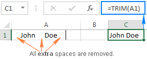
Yep, it’s that simple!
Please note that the TRIM function was designed to remove only the space character, which has value 32 in the 7-bit ASCII code system. If in addition to extra spaces, your data contains line breaks and non-printing characters, use the TRIM function in combination with CLEAN to delete the first 32 non-printing characters in the ASCII system.
For example, to remove spaces, line breaks and other unwanted characters from cell A1, use this formula:
=TRIM(CLEAN(A1))
For more information, please see How to remove non-printing characters in Excel
To get rid of nonbreaking spaces (html character ), which has value 160, use TRIM together with SUBSTITUTE and CHAR functions:
=TRIM(SUBSTITUTE(A1, CHAR(160), " "))
For full details, please see How to delete non-breaking spaces in Excel
How to use TRIM function in Excel – formula examples
Now that you know the basics, let’s discuss a few specific uses of TRIM in Excel, pitfalls that you may face and working solutions.
How to trim spaces in an entire column of data
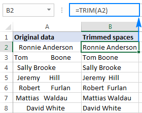
Supposing you have a column of names that have some whitespace before and after the text, as well as more than one spaces between the words. So, how do you remove all leading, trailing and excess in-between spaces in all cells at a time? By copying an Excel TRIM formula across the column, and then replacing formulas with their values. The detailed steps follow below.
- Write a TRIM formula for the topmost cell, A2 in our example:
=TRIM(A2) - Position the cursor to the lower right corner of the formula cell (B2 in this example), and as soon as the cursor turns into the plus sign, double-click it to copy the formula down the column, up to the last cell with data. As the result, you will have 2 columns – original names with spaces and formula-driven trimmed names.
- Finally, replace the values in the original column with the trimmed data. But be careful! Simply copying the trimmed column over the original column would destroy your formulas. To prevent this from happening, you need to copy only values, not formulas. Here’s how:
- Select all cells with Trim formulas (B2:B8 in this example), and press Ctrl+C to copy them.
- Select all cells with the original data (A2:A8), and press Ctrl+Alt+V, then V. It is the paste values shortcut that applies the Paste Special > Values
- Press the Enter key. Done!
How to remove leading spaces in a numeric column
As you have just seen, the Excel TRIM function removed all extra spaces from a column of text data without a hitch. But what if your data is numbers, not text?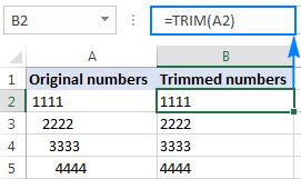
At first sight, it may seem that the TRIM function has done its job. Upon a closer look, however, you will notice that the trimmed values do not behave like numbers. Here are just a few indications of abnormality:
- Both the original column with leading spaces and trimmed numbers are left-aligned even if you apply the Number format to the cells, while normal numbers are right-aligned by default.
- When two or more cells with trimmed numbers are selected, Excel displays only COUNT in the status bar. For numbers, it should also display SUM and AVERAGE.
- A SUM formula applied to the trimmed cells returns zero.
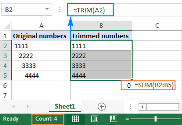
From all appearances, the trimmed values are text strings, while we want numbers. To fix this, you can multiply the trimmed values by 1 (to multiply all the values in one fell swoop, use the Paste Special > Multiply option).
A more elegant solution is enclosing the TRIM function in VALUE, like this:
=VALUE(TRIM(A2))
The above formula removes all leading and trailing spaces, if any, and turns the resulting value into a number, as shown in the screenshot below: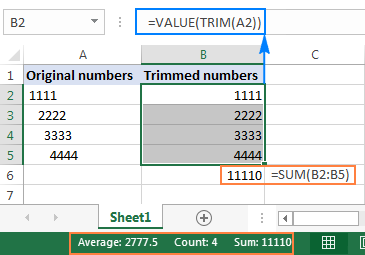
How to remove only leading spaces in Excel (Left Trim)
In some situations, you may type duplicated and even triplicated spaces between words to make your data better readable. However, you do want to get rid of leading spaces, like this: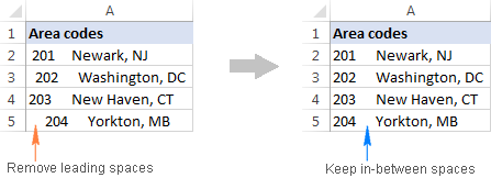
As you already know, the TRIM function eliminates extra spaces in the middle of text strings, which is not what we want. To keep all in-between spaces intact, we’ll be using a bit more complex formula:
=MID(A2,FIND(MID(TRIM(A2),1,1),A2),LEN(A2))
In the above formula, the combination of FIND, MID and TRIM calculates the position of the first text character in a string. And then, you supply that number to another MID function so that it returns the entire text string (the string length is calculated by LEN) starting at the position of the first text character.
The following screenshot shows that all leading spaces are gone, while multiple spaces between words are still there: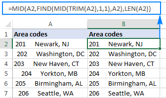
As a finishing touch, replace the original text with the trimmed values, as shown in step 3 of the Trim formula example, and you are good to go!
Tip. If you also want to remove spaces from the end of cells, make use of the Trim Spaces tool. There is no obvious Excel formula to remove leading and trailing spaces keeping multiple spaces between words intact.
How to count extra spaces in a cell
Sometimes, before removing spaces in your Excel sheet, you may want to know how many excess spaces are actually there.
To get the number of extra spaces in a cell, find out the total text length using the LEN function, then calculate the string length without extra spaces, and subtract the latter from the former:
=LEN(A2)-LEN(TRIM(A2))
The following screenshot shows the above formula in action: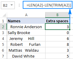
Note. The formula returns the count of extra spaces in a cell, i.e. leading, trailing, and more than one consecutive spaces between words, but it does not count single spaces in the middle of the text. If you want to get the total number of spaces in a cell, use this Substitute formula.
How to highlight cells with excess spaces
When working with sensitive or important information, you may be hesitant to delete anything without seeing what exactly you are deleting. In this case, you can highlight cells containing extra spaces first, and then safely eliminate those spaces.
For this, create a conditional formatting rule with the following formula:
=LEN($A2)>LEN(TRIM($A2))
Where A2 is the topmost cell with data that you want to highlight.
The formula instructs Excel to highlight cells in which the total string length is greater than the length of the trimmed text.
To create a conditional formatting rule, select all the cells (rows) that you want to highlight without column headers, go to the Home tab > Styles group, and click Conditional formatting > New Rule > Use a formula to determine which cells to format.
If you are not familiar with Excel conditional formatting yet, you will find the detailed steps here: How to create a conditional formatting rule based on formula.
As demonstrated in the screenshot below, the result perfectly corroborates with the extra spaces count that we got in the previous example: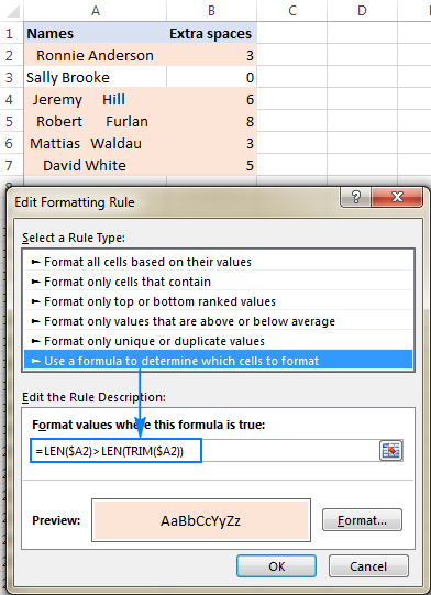
As you see, the use of the TRIM function in Excel is easy and straightforward.
Excel TRIM not working
The TRIM function only removes the space character represented by code value 32 in the 7-bit ASCII character set. In the Unicode character set, there is one more space character called the non-breaking space, which is commonly used on web pages as the html character . The nonbreaking space has a decimal value of 160, and the TRIM function cannot remove it by itself.
So, if your data set contains one or more white spaces that the TRIM function does not remove, use the SUBSTITUTE function to convert non-breaking spaces into regular spaces and then trim them. Assuming the text is in A1, the formula goes as follows:
=TRIM(SUBSTITUTE(A1, CHAR(160), " "))
As an extra precaution, you can embed the CLEAN function to clean the cell of any non-printable characters:
=TRIM(CLEAN(SUBSTITUTE(A1, CHAR(160), " ")))
The following screenshot shows the difference:
If the above formulas do not work for you either, chances are that your data contain some specific nonprinting characters with code values other than 32 and 160. In this case, use one of the following formulas to find out the character code, where A1 is a problematic cell:
Leading space: =CODE(LEFT(A1,1))
Trailing space: =CODE(RIGHT(A1,1))
In-between space (where n is the position of the problematic character in the text string):
=CODE(MID(A1, n, 1)))
And then, supply the returned character code to the TRIM(SUBSTITUTE()) formula discussed above.
For example, if the CODE function returns 9, which is the Horizontal Tab character, you use the following formula to remove it:
=TRIM(SUBSTITUTE(A1, CHAR(9), " "))
Trim Spaces for Excel – remove extra spaces in a click
Does the idea of learning a handful of different formulas to deal with a trivial task sound ridiculous? Then you may like this one-click technique to get rid of spaces in Excel. Let me introduce you to Trim Spaces tool included in our Ultimate Suite.
With Ultimate Suite installed in your Excel, removing spaces in Excel is as simple as this:
- Select the cell(s) where you want to delete spaces.
- Click the Trim Spaces button on the ribbon.
- Choose one or all of the following options:
- Trim leading and trailing spaces
- Trim extra spaces between words, except for a single space
- Trim non-breaking spaces ( )
- Click Trim.
That’s all there is to it! All extra spaces are removed in a blink.
In this example, we are only removing leading and trailing spaces, keeping multiple spaces between words intact for better readability – the task that Excel formulas cannot cope with is accomplished with a mouse click!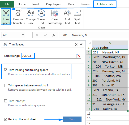
If you are interested to try Trim Spaces in your sheets, you are welcome to download an evaluation version at the end of this post.
I thank you for reading and look forward to seeing you next week. In our next tutorial, we will discuss other ways to trim spaces in Excel, please stay tuned!
If you need Microsoft Office 365, Genuine License product. must visit and order Now!
Microsoft Office 365 – 100% Genuine upgradeable license.
Powerful tools help you work, learn, organize, connect, and create.
–
Microsoft 365 – Available on your personal email.
Reinvent productivity with AI in Microsoft 365.
https://applecomputerspk.com/product/microsoft-365/
